Combining land cover and DEM

Create an elevation histogram for a particular land cover

Land cover data source: https://land.copernicus.eu/pan-european/corine-land-cover/clc2018

DEM data source: https://www.eea.europa.eu/data-and-maps/data/copernicus-land-monitoring-service-eu-dem

Reading and resampling

We want to be able to relate cells from one dataset to those of another. To do this the grids need to be ‘aligned’. We can do this by resampling both datasets onto the same grid. The simplest way to achive this is to resample one dataset onto the grid of the other dataset. In order to maintain the DEM’s higher resolution, we resample the land cover dataset onto the DEM’s grid.

The datasets can be large and we may not want to read the whole dataset into RAM if we don’t have to. We can supply a bounding box when reading the data to only read the data we need. If this bounding box is not defined in the coordinates native to the file, bounds_crs can be supplied to transform the bounds before reading. We can make use of this to read out a crop of the same area form different files.

Note

After reading a crop from a different CRS, the area is often not an exact match. When bounds are transformed to a different CRS, the bounds are warped. A bounding box is a rectagnle in it’s original CRS, but due to this warping it is often a paralellogram in a different CRS. In the current implementation, the furthest extent of the paralellogram define what data to crop. This means that more data is read when the bounds are warped more severely after the transformation.

import matplotlib.pyplot as plt
import numpy

from gridkit import read_raster

# Define the bounding box of interest and the corresponding CRS
bounds_matterhorn = (817723, 5826030, 964482, 5893982)
bounds_crs = 3857

# Define the paths to the data files
path_landuse = "../../tests/data/alps_landuse.tiff"
path_dem = "../../tests/data/alps_dem.tiff"

# Read a part of the digital elevation model (DEM) and set to desired CRS
dem = read_raster(path_dem, bounds=bounds_matterhorn, bounds_crs=bounds_crs)

# Read the same part of the landuse dataset and resample onto the DEM
landuse = read_raster(
    path_landuse, bounds=bounds_matterhorn, bounds_crs=bounds_crs
).resample(dem, method="nearest")

The resampling method ‘nearest’ was used to keep the land cover values discrete.

Tip

If you are unsure if your grids are aligned, you can put the resample step inside an if-statement. For this example that could look like so:

if not dem.is_aligned_with(landuse):
    landuse = landuse.resample(dem, method="nearest")

To get a feel for the area, I will plot the datasets side by side.

# Initialize figure for plotting the dem and landuse datasets
fig, axes = plt.subplots(2, constrained_layout=True)

# Plot DEM
im_dem = axes[0].imshow(dem, cmap="gist_earth", extent=dem.mpl_extent, aspect="auto")
fig.colorbar(im_dem, ax=axes[0], fraction=0.04, pad=0.01, label="Elevation [m]")
axes[0].set_ylabel("lat")
axes[0].set_title("Elevation [m]", fontsize=10)

# Plot Landuse
im_landuse = axes[1].imshow(
    landuse, cmap="tab20c_r", extent=landuse.mpl_extent, aspect="auto", vmin=0, vmax=50
)
fig.colorbar(im_landuse, ax=axes[1], fraction=0.04, pad=0.01, label="Landuse value")
axes[1].set_xlabel("lon")
axes[1].set_ylabel("lat")
axes[1].set_title("Landuse", fontsize=10)

plt.show()

To get a rough feeling for the land cover plot, the orange shades roughly correspond to snow, ice and bare rock and the green shades roughly correspond to vegetation. To inspect the land cover categories with better accuracy, visit the source of the data mentioned a the top of this page. You may notice the grey areas around the land cover dataset. These are nodata values used to fill empty areas during the resampling step.

Relating cells between datasets

To get the elevation distribution for a particular land cover we need to:

1. determine what cells hava a particular land cover

2. obtain the elevation values for these cells

3. plot the histogram

The first step is as simple as using a comparison operation on the grid. landuse == 1 will return the IDs of all cells where the land cover value is equal to 1. Since the landuse dataset has been resampled onto the grid of the DEM, the grids are ‘aligned’. This means we can simply use the IDs obtained from the landuse dataset to obtain the values of the DEM. First we obtain all ids in a dict. Then we loop through the dict and get the values from the dem grid using the ids obtains through the landuse grid.

from gridkit import index

# Determine elevation for the landuses of interest.
ids_per_landuse = dict(
    grass_and_shrub=index.concat([landuse == 26, landuse == 29]),
    bare_rock=landuse == 31,
    glacier=landuse == 34,
    conifer_forest=landuse == 24,
    mixed_forest=landuse == 25,
    broad_leaved_forest=landuse == 23,
)

Tip

Here the grass and shrub ids are combined using index.concat. Since the GridIndex returned by the comparison operation is based on numpy.ndarray, this is similar to calling numpy.vstack([landuse == 26, landuse == 29]). Naturally, the former will return a GridIndex and the latter a numpy ndarray. dem.value accepts either, so in this usecsae the two methods are equally viable.

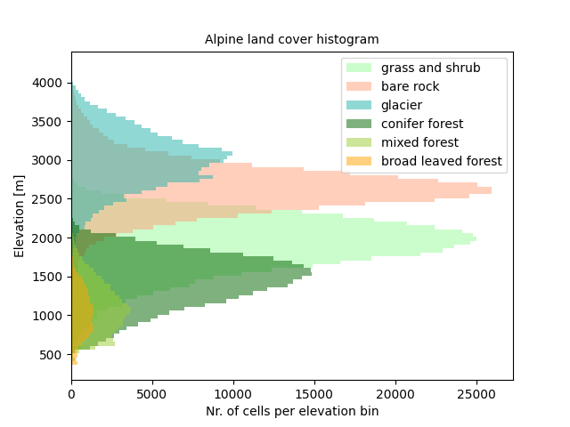
Plotting the histogram distribution of the various land covers gives the following plot:

# Plot forest histograms
fig, ax = plt.subplots(1)
bins = list(range(dem.min(), dem.max(), 50))
colors = iter(
    ["palegreen", "lightsalmon", "lightseagreen", "darkgreen", "yellowgreen", "orange"]
)
for name, ids in ids_per_landuse.items():
    ax.hist(
        dem.value(ids),
        bins=bins,
        color=next(colors),
        alpha=0.5,
        label=name.replace("_", " "),
        orientation="horizontal",
    )
ax.legend()
ax.set_xlabel("Nr. of cells per elevation bin")
ax.set_ylabel("Elevation [m]")
ax.set_title("Alpine land cover histogram", fontsize=10)
plt.show()