Coordinate transformations

Transform a grid from one CRS to another

Introduction

A Coordinate Reference System (CRS) is a means of representing a 3D surface (usually of Earth) onto a 2D map. There are many Coordinate Reference Systems, all with their own advantages and discrepencies. There is no one CRS to rule them all, there are only tradeoffs. That said, it is generally recommended to use a locally defined CRS when possible.

Note

In gridkit, a CRS is optional. If you represent, say, a generic image as a grid there is no need for a CRS. By default, the CRS property on a grid is None. It can either be supplied when the grid is initiated or by setting the propery on the grid after creation, e.g. grid.crs = 4326.

Warped grids

Grids always have straight lines in the CRS they are defined in. When a straigt line is transformed to a different CRS, it often gets warped. To demonstrate this, let’s create a grid in WGS84 (epsg code 4326) and transform the coordinates of each cell to CRS UTM N29 (epsg code 32629).

import numpy

from gridkit import BoundedRectGrid

# Create a new grid
grid_wgs84 = BoundedRectGrid(
    numpy.arange(25 * 25).reshape(25, 25),
    bounds=(-40, -30, 10, 20),
    crs=4236,
    nodata_value=numpy.nan,
).astype(
    "float32"
)  # use float dtype to be able to represent nans as nodata

# Plot the grid in it's native CRS
import matplotlib.pyplot as plt

plt.imshow(grid_wgs84, extent=grid_wgs84.mpl_extent)
plt.title("Original grid in WGS84")
plt.xlabel("$^\circ$Lon")
plt.ylabel("$^\circ$Lat")
plt.show()

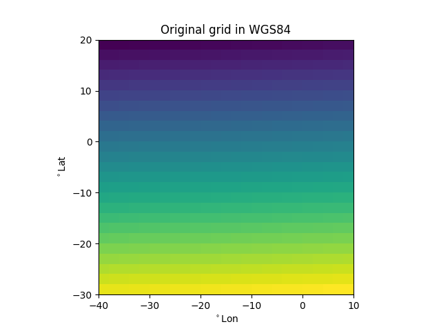
This is what the grid looks like it it’s native CRS. Now let’s transform the grid’s cell centers

from pyproj.transformer import CRS, Transformer

utm_epsg = 32629
transformer = Transformer.from_crs(
    grid_wgs84.crs, CRS.from_user_input(utm_epsg), always_xy=True
)  # UTM zone 28N

wgs84_centroids_utm = transformer.transform(
    *grid_wgs84.centroid().T
)  # transform each cell

# Plot the cell centers as a scatter plot, color them using their data value
plt.scatter(*wgs84_centroids_utm, s=20, c=grid_wgs84.data.ravel(), cmap="viridis")
plt.title("WGS84 grid cells transformed to UTM")
plt.xlabel("x [metre]")
plt.ylabel("y [metre]")
plt.show()

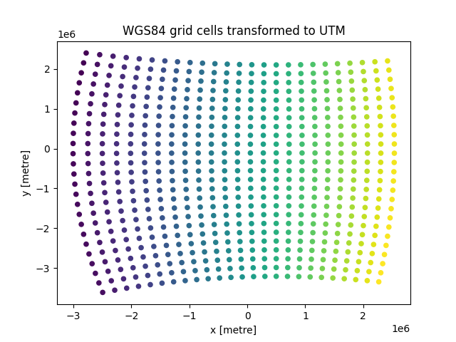
Notice how the whole grid is warped. There is nothing we can do to combat the warping. In order to work with a grid in a different CRS it needs to be resampled onto a grid that is straight in the new CRS. That is what happens when we call the to_crs() method on the grid. A new grid is crated that is straigt in the desired CRS. The values of the new grid cells are interpolated from the transformed values of the source grid. To demonstrate this principle, let’s plot the straight grid as red dots on top of the warped one, containing the original data.

grid_utm = grid_wgs84.to_crs(utm_epsg)  # resample using to_crs

# Plot the cells of the source grid in the new CRS
plt.scatter(*wgs84_centroids_utm, s=20, c=grid_wgs84.data.ravel(), cmap="viridis")
# Plot the location of the new cells
plt.scatter(*grid_utm.centroid().T, s=3, color="red")
plt.title("New UTM grid on top of WGS84 grid in UTM")
plt.xlabel("x [metre]")
plt.ylabel("y [metre]")
plt.show()

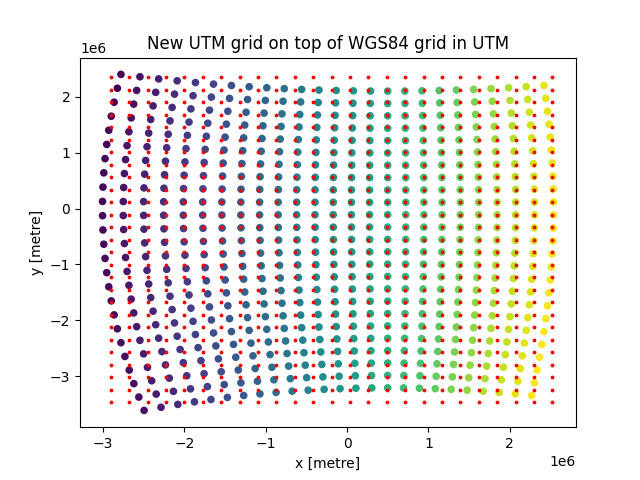
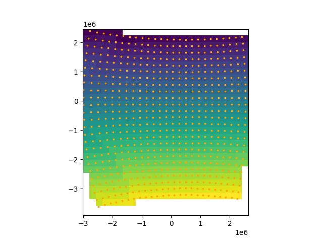
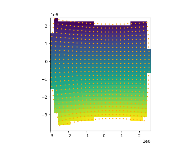
Now we showed only the location of the new grid cells, but when to_crs() was called, the data already got resampled. By default the ‘nearest’ resample_method is used. Let’s plot the new grid with the transformed WGS84 cell locations on top to see what happened.

plt.imshow(grid_utm, extent=grid_utm.mpl_extent)
plt.scatter(*wgs84_centroids_utm, s=3, color="orange")

plt.show()

For a smoother result, the ‘bilinear’ resample_method can be used. This does lead to artifacts at the boundaries.

grid_utm = grid_wgs84.to_crs(utm_epsg, resample_method="bilinear")
plt.imshow(grid_utm, extent=grid_utm.mpl_extent)
plt.scatter(*wgs84_centroids_utm, s=3, color="orange")

plt.show()

to_crs() is just a shorthand for creating a grid with the same properties as the source grid, but with a different CRS, and calling resample. Any time source_grid.resample(target_grid) is called, the CRS of the grids are compared. If they are different, the logic described in this example is applied.