Downslope path

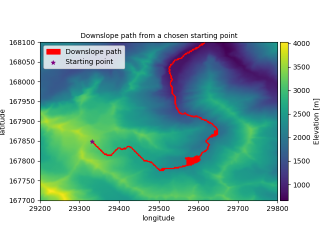
Use a DEM to determine the downslope path from a point on the DEM to the edge.

DEM data source: https://www.eea.europa.eu/data-and-maps/data/copernicus-land-monitoring-service-eu-dem

Introduction

In this example the downslope path is found from a given point on a DEM. This can be conceptualized as the path water would flow donw from a given source. This algorithm does not stop at a local minimum, but continues when the edge of the DEM is reached. The path can therefore be best conceptualized as a stram, possibly with small lakes, rather than a single droplet.

Method

This is done by iteratively finding the neighbour with the lowest elevation.

In this example, the flow is as follows:

1. A cell is supplied to the “downslope_path” function

2. The neighbouring cells are obtained

3. These cells are added to a list containing all neighbours along the path so far

4. The neighbour along the path so far with the lowest elevation is added to the path, at which point we start again at 1.

The loop stops when NaNs are encountered, which happens when the border of the DEM crop is reached. This is of course assuming there are no nodata_values in the DEM.

First let’s import the dependencies and read in the DEM.

import matplotlib.pyplot as plt
import numpy

from gridkit import read_raster

dem = read_raster(
    "../../tests/data/alps_dem.tiff", bounds=(29200, 167700, 29800, 168100)
)

Next, set up the recursive function and the required empty lists.

Warning

Python’s recursion limit can be reached with this approach for paths longer than shown here. While you can raise this limit using sys.setrecursionlimit, you may want to reconsider the approach and use a while-loop instead of recursion.

visited_cells = []
all_neighbours = []
neighbour_values = []


def downslope_path(cell_id):
    visited_cells.append(cell_id)
    # add new neigbours and their values to their respective lists
    neighbours = dem.neighbours(cell_id, connect_corners=True)
    for cell, value in zip(neighbours, dem.value(neighbours)):
        cell = tuple(cell.index)
        if not cell in visited_cells and not cell in all_neighbours:
            all_neighbours.append(cell)
            neighbour_values.append(value)

    # stop when we encounter nodata values, assuming these only occur byound the bounds of the DEM crop
    if dem.nodata_value in neighbour_values:
        return

    # determine the next cell and remove it from the neighbour-lists
    min_id = numpy.argmin(neighbour_values)
    next_cell = all_neighbours[min_id]
    all_neighbours.pop(min_id)
    neighbour_values.pop(min_id)

    return downslope_path(next_cell)

Determine the starting cell and call the function

start_cell_id = dem.cell_at_point((29330, 167848))
downslope_path(tuple(start_cell_id.index))

Results

Let’s plot the path on the DEM

For each cell along the path we plot the polygon as a square. This looks better than points at the centroids.

im = plt.imshow(dem, extent=dem.mpl_extent)
plt.colorbar(fraction=0.032, pad=0.01, label="Elevation [m]")
plt.xlabel("longitude")
plt.ylabel("latitude")
plt.title("Downslope path from a chosen starting point", fontsize=10)

path_label = "Downslope path"
for poly in dem.to_shapely(visited_cells):
    x, y = poly.exterior.xy
    plt.fill(x, y, alpha=1.0, color="red", label=path_label)
    path_label = None  # Only show the label in the legend once

plt.scatter(
    *dem.centroid(start_cell_id), marker="*", label="Starting point", color="purple"
)
plt.legend()

plt.show()

While the path is merely visualized in this example, the obtained cells can of course be used in different ways. They can for example be used to obtain values form a different dataset along the path, or intersected with a polygon to determine if the path crosses a particular zone of interest.