2D Diffusion

2D Diffusion on a HexGrid

Introduction

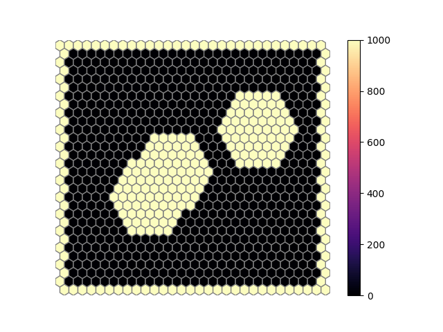
This example shows basic 2D diffusion on a HexGrid. We start with a cold region surrounded by hot borders. We will also add some hot patches in the middle of the cold region to make it look interesting. The heat is then spread out by diffusion.

Diffusion

Diffusion is a description of the spread of a physical property through time. An easy example is the spread of temperature, which is what we will use in this example, but other physical properties can also be modelled using diffusion. Diffusion is often coupled with advection (the transport of a substance) in models of fluid flow. Here we will only focus on the diffusion.

1D diffusion equation derivation

First I will derive the diffusion equation for one dimension, and then extrapolate to multiple dimensions.

Let’s start by viewing the distribution of temperature in a given space as being divided into many small regions where the temperature is the same. I will call such a region a control volume. Such a volume can conceptually be infinitesimally small, but for modelling purposes these control volumes will be given a finite size. The change of the temperature (\(\Delta T\)) in a given control volume is determined by the temperature flux going in to the control volume (\(T_{flux}^{in}\)) minus the temperature flux leaving the control volume (\(T_{flux}^{out}\)) in a given time step \(\Delta t\).

This means that the temperature in the next time step (\(T^{t+\Delta t}\)) is determined by the current temperature (\(T^t\)) and the fluxes. As an equation this looks like:

\[T^{t+\Delta t} = T^{t} + \Big( T_{flux}^{in} - T_{flux}^{out} \Big) \Delta t\]

or equivalently:

\[T^{t+\Delta t} - T^{t} = \Big( T_{flux}^{in} - T_{flux}^{out} \Big) \Delta t\]

\(T_{flux}^{in}\) and \(T_{flux}^{out}\) describe the same kind of flux, but at different locations in space, separated in space by distance \(\Delta x\). Let’s rewrite this as:

\[T^{t+\Delta t} - T^{t} = \Big( [ T_{flux} ] ^{x} - [ T_{flux} ] ^{x + \Delta x} \Big) \Delta t\]

The temperature flux, or heat flux, has a unit of energy per unit area per unit time. I will take a bit of a shortcut and say that the heat flux is given by:

\[T_{flux} = D \frac{ \Delta T }{ \Delta x \Delta t }\]

Where \(D\) is the thermal diffusivity, which a constant and is dependent to the thermal conductivity of the material.

Substituting this into the equation above it we get:

\[T^{t+\Delta t} - T^{t} = \Big( \Big[ D \frac{ \Delta T }{ \Delta x \Delta t } \Big] ^{x} - \Big[ D \frac{ \Delta T }{ \Delta x \Delta t } \Big] ^{x + \Delta x} \Big) \Delta t\]

which we can simplify as:

\[T^{t+\Delta t} - T^{t} = D \frac{ \Delta T^x - \Delta T^{x+\Delta x} } {\Delta x}\]

Here, \(T^{t+\Delta t} - T^{t}\) describes a change in temperature over a given time period \(\Delta t\). This can also be written as \(\frac{ \Delta T }{ \Delta t }\). Similarly, \(\Delta T^x - \Delta T^{x+\Delta x}\) describes a change in temperature over a given distance \(\Delta x\), which can also be written as \(\frac{ \Delta T }{ \Delta x }\). We can therefore rewrite the equation given above as:

\[\frac{ \Delta T }{ \Delta t } = D \frac{ \frac{ \Delta T }{ \Delta x } }{ \Delta x }\]

or equivalently:

\[\frac{ \Delta T }{ \Delta t } = D \frac{ \Delta T }{ \Delta x \Delta x }\]

If we have \(\Delta t\) and \(\Delta x\) tend to zero, we can write this as the differential equation:

\[\frac{ \delta T }{ \delta t } = D \frac{ \delta ^2 T }{ \delta x^2 }\]

This is the basic form of the 1D thermal diffusion equation.

Multi-dimensional diffusion equation

Usually, the 1D diffusion equation described above is extrapolated to 2D by considering two perpendicular directions of flow, dx and dy. The diffusion equation then becomes:

\[\frac{ \delta T }{ \delta t } = D \Big( \frac{ \delta ^2 T }{ \delta x^2 } + \frac{ \delta ^2 T }{ \delta y^2 } \Big)\]

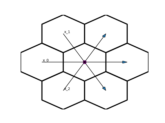
This works nicely for rectangular grids, but since we will be using a hexagonal grid in this example, this won’t do nicely. We will have to describe the directions in terms of the surrounding cells. Since a hexagon has 6 surrounding cells, we can describe the total flow as having three directions in a 2D plane. To demonstrate what I mean, I will create a plot demonstrating the flow in three directions, x1, x2 and x3:

import matplotlib.pyplot as plt

from gridkit import GridIndex, HexGrid
from gridkit.doc_utils import plot_polygons

grid = HexGrid(size=1)
ids = grid.neighbours([0, 0])
centroids = grid.centroid(ids.sort())

plot_polygons(grid.to_shapely(ids), fill=False, linewidth=3)
plt.scatter(
    *grid.centroid([0, 0]), marker="h", color="purple", s=100
)  # plot center, indicating location of temperature
for i in range(3):
    from_ = centroids[0 + i]
    to = centroids[5 - i]
    # to = centroids[3+i]
    plt.arrow(
        *from_, *(to - from_), head_width=0.07, overhang=-0.1, length_includes_head=True
    )
    plt.text(*centroids[0 + i] + 0.02, f"x_{i}")
plt.axis("off")
plt.show()

Using these three directions, we can modify the diffusion equation appropriately:

\[\frac{ \delta T }{ \delta t } = D \Big( \frac{ \delta ^2 T }{ (\delta (x_1)^2 } + \frac{ \delta ^2 T }{ (\delta x_2) ^2 } + \frac{ \delta ^2 T }{ (\delta x_3)^2 } \Big)\]

We can apply the ‘forward time-centered space’ finite difference method to this equation to get a form we can run as code. This approach uses the flux on both boundaries of the cell. In 1D this looks like so:

\[T_{x}^{t_{n+1}} = T_{x}^{t_n} + D \Delta t \frac{ T_{x+1}^{t_n} - 2T_{x}^{t_n} + T_{x-1}^{t_n} }{ \Delta x^2 }\]

Here \(T_{x}^{t_{n+1}}\) is the temperature at location x` for the next time step (\(t_{n+1}\)), which is a function of the temperature at location x (\(T_{x}^{t_n}\)) at the current time step () (\(t_n\)) and that of the cells at locations \(x-1\) and \(x+1\).

For the multi-dimensional case using x1, x2 and x3, this equation becomes:

\[\begin{split}T_{x}^{t_{n+1}} = T_{x}^{t_n} + D \Delta t \Big( \\ \frac{ T_{x_0+1, x_1, x_2}^{t_n} - 2T_{x_0, x_1, x_2}^{t_n} + T_{x_0-1, x_1, x_2}^{t_n} }{ (\Delta x_0)^2 } + \\ \frac{ T_{x_0, x_1+1, x_2}^{t_n} - 2T_{x_0, x_1, x_2}^{t_n} + T_{x_0, x_1-1, x_2}^{t_n} }{ (\Delta x_1)^2 } + \\ \frac{ T_{x_0, x_1, x_2+1}^{t_n} - 2T_{x_0, x_1, x_2}^{t_n} + T_{x_0, x_1, x_2-1}^{t_n} }{ (\Delta x_2)^2 } \Big)\end{split}\]

Now, I realize this might look intimidating if you are not used to big equations. Luckily we can simplify this. By the definition of our hexagonal grid, the distances \((\Delta x_0)^2\), \((\Delta x_1)^2\) and \((\Delta x_2)^2\) are all the same. Since all these distances are that of the cell width from side to side, let’s call this distance cell_width. This means the equation can be written as:

\[\begin{split}&T_{x}^{t_{n+1}} = T_{x}^{t_n} + \\ &D \Delta t \Big(\frac{ T_{x_0+1, x_1, x_2}^{t_n} + T_{x_0-1, x_1, x_2}^{t_n} + T_{x_0, x_1+1, x_2}^{t_n} + T_{x_0, x_1-1, x_2}^{t_n} + T_{x_0, x_1, x_2+1}^{t_n} + T_{x_0, x_1, x_2-1}^{t_n} - 6T_{x_0, x_1, x_2}^{t_n} }{ cell\_width^2 } \Big)\end{split}\]

Looking closely at the top of the numerator, one might observe this is basically a matter of adding the temperatures of all six neighbours and subtracting the temperature of the center cell six times. Taking some artistic liberty with mathematical notation, this can then be written as:

\[T_{x}^{t_{n+1}} = T_{x}^{t_n} + D \Delta t \Big(\frac{ \sum_{i=0}^{6} T_{neighbour\_i}^{t_n} - 6T_{x_0, x_1, x_2}^{t_n} }{ cell\_width^2 } \Big)\]

Here \(T_{neighbour\_i}^{t_n}\) refers to the temperature of the ‘i-th’ neighbour, of which there are six.

Finally, the step size in time \(\Delta t\) is determined by the following equation:

\[\Delta t = \frac{1}{2D} \frac{ (\Delta x_0 \Delta x_1 \Delta x_2)^2 }{ ( \Delta x_0)^2 + (\Delta x_1)^2 + (\Delta x_2)^2 }\]

Which we can simplify to:

\[\Delta t = \frac{1}{2D} \frac{ cell\_width^6 }{ 3 (cell\_width^2) }\]

and further to:

\[\Delta t = \frac{ cell\_width^4 }{ 6 D }\]

Setup

Now we have the theory covered, let’s define a setup with some parameters. The setup is inspired by the following article: https://scipython.com/book/chapter-7-matplotlib/examples/the-two-dimensional-diffusion-equation/ Though we will modify it a bit, to make it look a bit more interesting. First, let’s define a region and divide that up in hexagons.

# Grid size
grid = HexGrid(size=1)  # Define grid in mm
nr_cells_x = nr_cells_y = 30

# Thermal properties
D = 4.0  # Thermal diffusivity of steel, mm2.s-1
Tcool, Thot = 0, 1000  # Temperatures in degrees

# plotting
plot_interval = 0.1  # time in seconds
tmax = 1.0  # time in seconds

For the boundary conditions, we will have a hot rim surrounding the modelled area. Let’s define the outer bounds and the inner bounds, where the inner bounds will be cool, and the cells between the inner bound and outer bound are hot. The hot cells at the boundary will remain hot and will not be updated in the time loop.

outer_bounds = (0, 0, nr_cells_x * grid.dx, nr_cells_y * grid.dy)
inner_bounds = (
    grid.dx,
    grid.dy,
    (nr_cells_x - 1) * grid.dx,
    (nr_cells_y - 1) * grid.dy,
)
inner_ids = grid.cells_in_bounds(inner_bounds).ravel()

datagrid = grid.to_bounded(outer_bounds, fill_value=Thot)
np_ids = datagrid.grid_id_to_numpy_id(inner_ids)
datagrid.data[np_ids] = Tcool

Also, let’s select some cells form inside the cold region and give them a hot starting temperature to make it look more interesting.

hot_ids = (
    grid.neighbours([[9, 11], [12, 14], [21, 19]], depth=4, include_selected=True)
    .ravel()
    .unique()
)
np_ids_hot = datagrid.grid_id_to_numpy_id(hot_ids)
datagrid.data[np_ids_hot] = Thot

Let’s take a look at what these starting conditions look like

plot_polygons(
    datagrid.to_shapely(),
    colors=datagrid.data.ravel(),
    fill=True,
    cmap="magma",
    edgecolor="grey",
    add_colorbar=True,
)
plt.axis("off")
plt.show()

Here, all beige cells are the cells that start out hot and the black cells start out cool.

The model

For this grid, the important variables we will need for the diffusion equation are:

cell_width = grid.dx
dt = cell_width**4 / (6 * D)

We will only have to obtain the neighbour indices once and reuse these every time step.

neighbours = grid.neighbours(inner_ids)
nbr_ids = neighbours.index

It’s finally time to do the real work. Loop through time, solve the diffusion equation and save the intermediate data for later plotting:

time = 0
time_since_last_plot = plot_interval  # start with a plot of the initial state
plot_data = []
plot_titles = []
while time < tmax:
    if time_since_last_plot >= plot_interval:  # Save data every plot_interval
        plot_data.append(datagrid.data.ravel().copy())
        plot_titles.append("{:.1f} ms".format(time * 1000))
        time_since_last_plot = 0
    # Solve diffusion equation for this timestep
    datagrid.data[np_ids] = datagrid.data[np_ids] + D * dt * (
        (datagrid.value(nbr_ids).sum(axis=-1) - 6 * datagrid.value(inner_ids))
        / cell_width**2
    )
    time += dt
    time_since_last_plot += dt

Animation

from matplotlib.animation import FuncAnimation

all_geoms = datagrid.to_shapely()


def update_frame(frame_id):
    ax.clear()
    im = plot_polygons(
        all_geoms,
        colors=plot_data[frame_id],
        fill=True,
        ax=ax,
        cmap="magma",
        vmin=Tcool,
        vmax=Thot,
    )
    ax.set_title(plot_titles[frame_id])
    ax.set_aspect("equal")
    ax.set_axis_off()


# Create animation
fig, ax = plt.subplots()
anim = FuncAnimation(
    fig, update_frame, frames=range(0, len(plot_data)), repeat=True, interval=200
)
plt.show()

Once Loop Reflect