Cellular automata: Conway’s game of life

Cellular automata are a small set of rules relating to cells on a grid that can create complex patterns when applied repeatedly. There is a near infinite veriety of rules, but far and away the most well known set of rules is that of the so called Conway’s game of life. The setup is as follows:

• The board is a 2d rectangular grid

• The 8 neighbouring cells are considered, so this includes the diagonal neighbours

• A cell has two possbile states: alive or dead

The rules as taken from https://en.wikipedia.org/wiki/Conway%27s_Game_of_Life:

1. Any live cell with fewer than two live neighbours dies, as if by underpopulation.

2. Any live cell with two or three live neighbours lives on to the next generation.

3. Any live cell with more than three live neighbours dies, as if by overpopulation.

4. Any dead cell with exactly three live neighbours becomes a live cell, as if by reproduction.

Initial conditions

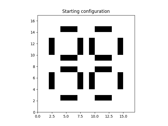
All cellular automata simulations are highly dependent on the initial conditions. We have to start with some dead cells and some live cells. After all, according to these rules, if all cells are live, the cells will die in the next generation and if all cells are dead, they stey dead for they would need three live neighbours to become a live cell. Therefore we need to start with something that is at least halfway interesting. Let’s set up a starting scenario. Feel free to download this script as a notebook and start fiddeling yourself. The particular starting scenario I chose will replicate itself in three generations, which makes it convenient for creating a looping animation.

import matplotlib.pyplot as plt
import numpy

from gridkit import BoundedRectGrid
from gridkit.doc_utils import plot_polygons

# Initialize
shape = (17, 17)
data = numpy.zeros(shape)
data[2, 4:7] = 1
data[2, 10:13] = 1
data[7, 4:7] = 1
data[7, 10:13] = 1
data[9, 4:7] = 1
data[9, 10:13] = 1
data[14, 4:7] = 1
data[14, 10:13] = 1
data[4:7, 2] = 1
data[10:13, 2] = 1
data[4:7, 7] = 1
data[10:13, 7] = 1
data[4:7, 9] = 1
data[10:13, 9] = 1
data[4:7, 14] = 1
data[10:13, 14] = 1

grid = BoundedRectGrid(data=data)

neighbours = grid.neighbours(grid.indices, connect_corners=True)
neighbours = neighbours = numpy.stack(
    grid.grid_id_to_numpy_id(neighbours.ravel())
).T.reshape((*shape, 8, 2))

plt.imshow(grid, extent=grid.mpl_extent, cmap="gray_r")
plt.title("Starting configuration")
plt.show()

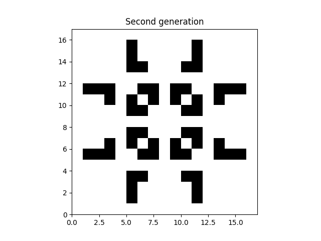
The naive method

We can convert the rules into code. The naive but intuitive way would look something like:

data_second_gen = data.copy()
for i in range(1, shape[0] - 1):
    for j in range(1, shape[1] - 1):
        nb = neighbours[i, j]
        nr_nb_live = data[nb.T[0], nb.T[1]].sum()
        if data[i, j] == 1:  # live cell
            if nr_nb_live == 2 or nr_nb_live == 3:
                data_second_gen[i, j] = 1
            else:
                data_second_gen[i, j] = 0
        else:  # Dead cell
            if nr_nb_live == 3:
                data_second_gen[i, j] = 1
            else:
                data_second_gen[i, j] = 0

plt.imshow(data_second_gen, extent=grid.mpl_extent, cmap="gray_r")
plt.title("Second generation")
plt.show()

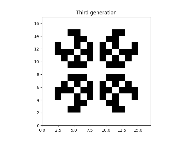
The performant method

The unfortunate thing about this method is that it loops over all cells in python, which is slow. As a first optimization we can get rid of the conditionals by adding all the contributions. This can looks something like:

data_third_gen = data.copy()
for i in range(1, shape[0] - 1):
    for j in range(1, shape[1] - 1):
        nb = neighbours[i, j]
        nr_nb_live = data_second_gen[nb.T[0], nb.T[1]].sum()
        data_third_gen[i, j] = (
            0
            + (data_second_gen[i, j] == 1) * (nr_nb_live == 2 or nr_nb_live == 3)
            + (data_second_gen[i, j] != 1) * (nr_nb_live == 3)
        )

plt.imshow(data_third_gen, extent=grid.mpl_extent, cmap="gray_r")
plt.title("Third generation")
plt.show()

With the code written like this, it is clear that we can also remove the double python loop by utilizing numpy slices:

nb = data_third_gen[
    neighbours[1 : shape[0] - 1, 1 : shape[1] - 1, :, 0],
    neighbours[1 : shape[0] - 1, 1 : shape[1] - 1, :, 1],
]
nr_nb_live = nb.sum(axis=-1)
is_live = data[1 : shape[0] - 1, 1 : shape[1] - 1] == 1
data_fourth_gen = (
    0 + is_live * ((nr_nb_live == 2) | (nr_nb_live == 3)) + ~is_live * (nr_nb_live == 3)
)

plt.imshow(data_fourth_gen, extent=grid.mpl_extent, cmap="gray_r")
plt.title("Fourth generation")
plt.show()

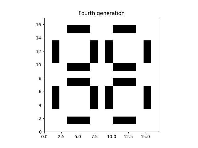
Note how this fourth generation looks the same as the starting conditions. The pattern loops every three frames/generations.

Written this way, you could even run this logic on a GPU using PyTorch or wgpu, but since most time is now spent plotting using matplotlib you might also want to consider a different visualization method (for example py-gfx) if a speedup for larger grids is desired.

Animation

Since we are iterating over time, cellular automata lend itself well for an animation. Given the logic above, the animation code can look like so:

def update_frame(frame):
    nb = data[
        neighbours[1 : shape[0] - 1, 1 : shape[1] - 1, :, 0],
        neighbours[1 : shape[0] - 1, 1 : shape[1] - 1, :, 1],
    ]
    nr_nb_live = nb.sum(axis=-1)
    is_live = data[1 : shape[0] - 1, 1 : shape[1] - 1] == 1
    data[1 : shape[0] - 1, 1 : shape[1] - 1] = (
        0
        + is_live * ((nr_nb_live == 2) | (nr_nb_live == 3))
        + ~is_live * (nr_nb_live == 3)
    )
    ax.clear()
    ax.imshow(data, extent=grid.mpl_extent, cmap="gray_r")
    ax.set_title(frame)
    ax.set_axis_off()


# Create animation
from matplotlib.animation import FuncAnimation

fig, ax = plt.subplots()
ax.set_aspect("equal")
ax.imshow(data, extent=grid.mpl_extent, cmap="gray_r")
anim = FuncAnimation(fig, update_frame, frames=range(0, 6), repeat=True, interval=300)
plt.show()

Once Loop Reflect